Yolov7: Artificial Intelligence for real-time object detection in an image

In this article we will discover the Yolov7 model, an object detection algorithm. We will first study its use and its characteristics through a public dataset. Then we will see how to train this model ourselves from this dataset. Finally, we will train Yolov7 to identify custom objects from our own data.

What is Yolo? Why Yolov7 ?

Yolo is an algorithm for detecting objects in an image. The goal of object detection is to automatically classify, using a neural network, the presence and position of humanly identifiable objects in an image. The interest is therefore based on the capacities and performances in terms of detection, recognition and localization of the algorithms, which have multiple practical applications in the image domain. Yolo's strength lies in its ability to perform these tasks in real time, which makes it particularly useful with video streams of tens of images per second.

YOLO is actually an acronym for "You Only Look Once". Indeed, unlike many detection algorithms, Yolo is a neural network that evaluates the position and class of identified objects from a single end-to-end network that detects classes using a fully connected layer. Yolo therefore only needs to "see" an image once to detect the objects present, where some algorithms only detect regions of interest, before re-evaluating these to identify the classes present. Before mentioning the other versions of Yolo, it seems important here to explain the different metrics used to compare the accuracy and efficiency of a model.

Intersection over Union : IoU

Intersection over Union (literally Intersection over Union, or IoU) is a metric for measuring the accuracy of object location. As its name indicates, it is calculated from the ratio between the intersection area of the detected object and the union area of these same objects (see equation 1). By noting Adetected and Aactual the respective areas of the object detected by YOLO and the object as actually located on the image, we can then write :

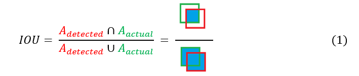
Note that an IoU of 0 indicates that the 2 areas are completely distinct and that an IoU of 1 indicates that the 2 objects are perfectly superimposed. In general, an IoU > 0.5 represents a valid localization criterion.

(mean) Average Precision : mAP

Average Precision is a classification accuracy metric. It is based on the average of the correct predictions over the total predictions. So we try to get closer to a 100% mAP score (no error when determining the class of an object).

Coming back to our previous point, Yolo remains an architecture model, and not the property of a particular developer. This explains why the versions of Yolo are from different contributors. Indeed, we increment the version of Yolo (Yolov7 to date: January 2023) each time the previously mentioned metrics (especially the mAP and its associated execution time) clearly exceed the previous model and thus the state of the art. Thus, each new YolovX model is actually an improvement shown by an associated research paper published in parallel.

How does Yolo work?

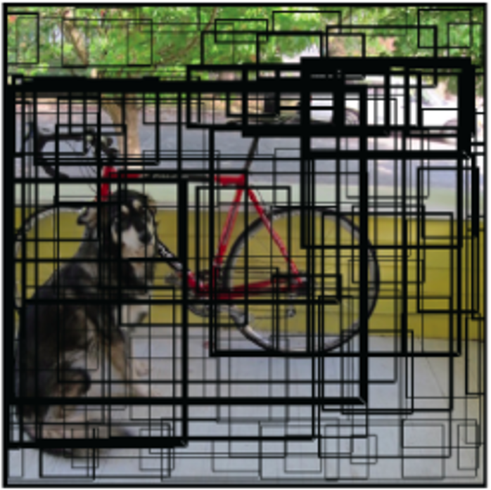
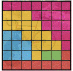
Yolo works by segmenting the image that it analyzes. It will first grid the space, then perform 2 operations: localization and classification.

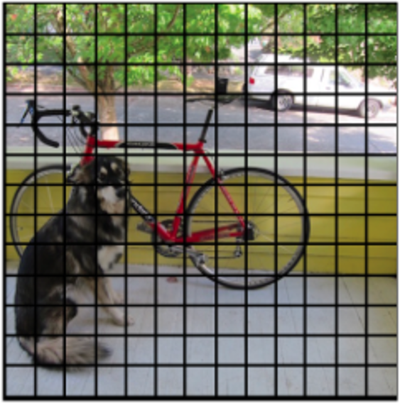
First, Yolo identifies all the objects present with the help of frames by associating them a degree of confidence (here represented by the thickness of the box).

Then, the algorithm assigns a class to each box according to the object that it believes it has detected from the probability map.

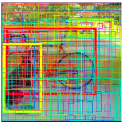
Finally, Yolo removes all unnecessary boxes using the NMS method.

NMS : Non-Maxima Suppression

The NMS method is based on a path of the high confidence index boxes, then a removal of the boxes superimposed on those by measuring the IoU. For this, we follow 4 steps. Starting from the complete list of detected boxes:

1. Remove all boxes with a low confidence index.
2. Identification of the box with the highest confidence index.
3. Deleting all boxes with too large IoU (i.e. all boxes too similar to our reference box).
4. Ignoring the reference box thus used, repeat steps 2) and 3) until all boxes in our original list have been eliminated (i.e. taking the 2nd largest confidence index box, then the 3rd, etc.).

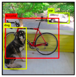
We then obtain the following result:

How to use Yolov7 with the COCO dataset ?

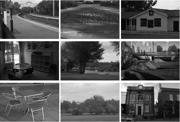
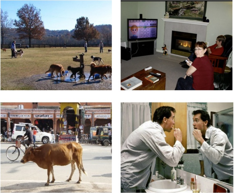
Now that we have seen the Yolo model in detail, we will study its use with an image database: the COCO dataset. The MICROSOFT COCO dataset (for Common Objects in COntext), more commonly called MS COCO, is a set of images representing common objects in a common context. However, unlike the usual databases used for object detection and recognition, MS COCO does not present isolated objects or scenes. Indeed, the goal when creating this dataset was to have images close to real life, in order to have a more robust training base for classical image streams, reflecting daily life.

Thus, by training our Yolov7 model with the MS COCO dataset, it is possible to obtain a recognition algorithm of nearly a hundred classes and categorizing the majority of objects, people and elements of everyday life. Finally, MS COCO is today the main reference for measuring the accuracy and efficiency of a model. To get an idea, below are the results of the different versions of Yolo.

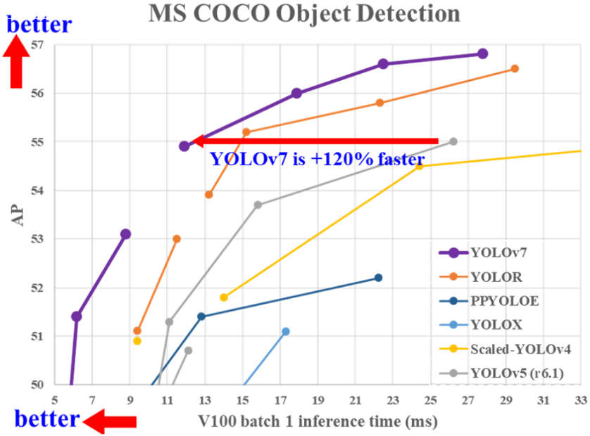
On the x-axis, the times given to the networks to evaluate an image are indicated. The lower the time, the more we can afford to send a large flow of images to our algorithm, at the cost of accuracy. On the ordinate, the average accuracy of the models is indicated as a function of the time allowed, as seen previously.

We then notice 3 important points:

1. Regardless of the time given to the network, Yolov7 outperforms the other Yolo models in terms of detection accuracy on the MS COCO dataset. This explains its presence as a reference in the current state of the art of real-time image-based object detection.
2. The increase of the inference time on each image has no/few interest once the 30ms/image is exceeded. This implies that the model is more optimal on a use requiring fast image processing, such as a video stream (> 25 fps).
3. Regardless of the model concerned, none of them exceeds 57% of detection accuracy. This implies that the model is still far from being able to be used reliably in a public setting.

To obtain the above results yourself, just follow the instructions on the GitHub page of the yolov7 model pre-trained from the MS COCO dataset: https://github.com/WongKinYiu/yolov7.

First, follow the heading :

• Installation.

Then the sidebar:

• Testing.

How to train Yolov7 ?

Now that we have seen how to test Yolov7 with a dataset on which it is trained, we are going to look at how we can train Yolov7 with our own dataset. We will first start a training with already prepared data, here the MS COCO dataset. Again, the Yolov7 GitHub has a specific insert for this purpose:

• Training.

It is broken down into 2 simple steps:

1. Download the already annotated MS COCO dataset.
2. Launch the script " train.py " intrinsic to the Git directory with the dataset previously downloaded.

This one will then run on 300 steps to conform to the MS COCO dataset. It should be noted that in reality this operation has more of an instructive purpose since Yolov7 is already trained on the MS COCO dataset and thus already has an adequate model.

Prepare your own training data

Now that we have seen what Yolov7 is, how to test it and train it, we just have to provide it with our own image base to train it on our use case. We will therefore follow 4 steps to create our own dataset directly usable to train Yolov7 :

1. Choice of our image database.
2. Optional: Labeling of all our images.
3. Preparation of the launch (use case of Google Collab).
4. Training (and split operation).

To illustrate the sequence of these operations, we will take a case similar to the Novelis work used on AIDA: the detection of elements drawn on a sheet of paper.

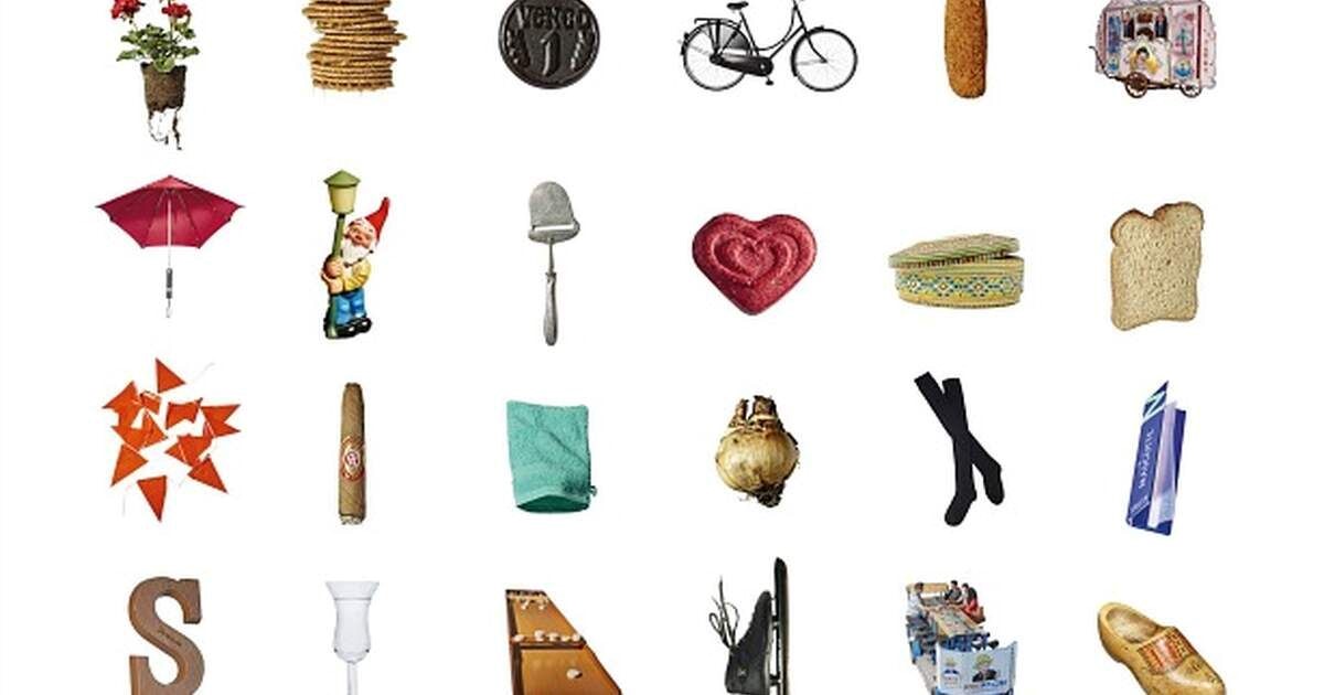
To start, we will need to get a sufficient quantity of similar images. Either from our own collection, or by using a pre-existing database (for example by taking the dataset of our choice from this link. On our part, we will use the Quick Draw dataset. Once our database is formed, we will annotate our images. For that, many softwares exist, most of the time allowing to create boxes, or polygons, and to label them as a class. In our case, our database is already labeled, otherwise we would have to create a class for each element to be detected, and then identify by hand on each image the exact areas of presence of these classes. Once our dataset is labelled, we can launch a session on Google Colab and start a new Python Notebook. We will call it "MyYolov7Project.ipynb" for example.

First step: copy your dataset in your drive. In our case, we have already added to our drive a folder "Yolov7_Dataset". Here is the tree structure of the folder:

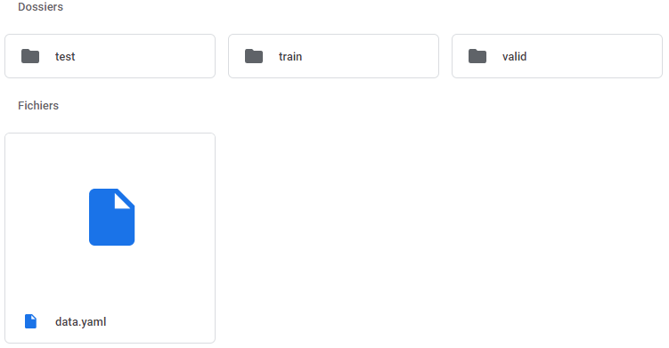
For each folder, there is an images folder, containing the images, and a labels folder containing the associated labels generated previously. In our case, we use 20 000 images in total, including 15 000 for training, 4 000 for validation and 1 000 for testing.

The data.yaml file contains all the paths to the :

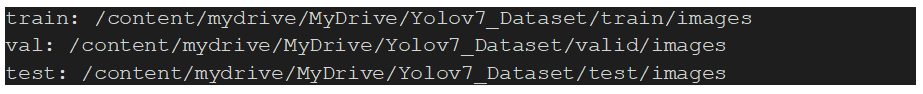
Then the characteristics of the classes:

We will not show the 345 classes in detail but they should be present in your file. We can now start our script "MyYolov7Project.ipynb" on Colab. First step, link our Drive to Colab in order to save our results (Be careful : the data of the trained network are voluminous).

Once our Drive is linked, we can now clone Yolov7 from the official Git:

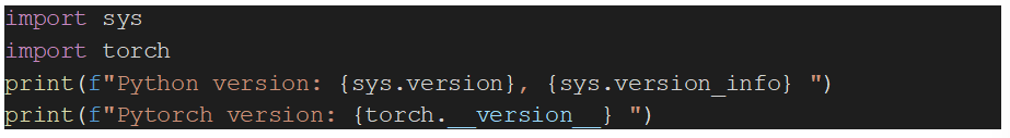
By placing us in the installed folder, we check the prerequisites:

We will also need the sys and torch libraries.

We can then run the training script for our network:

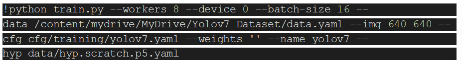
Note that the batch size can be modified according to the capacities of your GPU (with the free version of Collab, 16 is the maximum possible). Don't forget to modify your path to the "data.yaml" file according to the tree structure of your Drive. At the end of the training, we get a file with the training metrics and a trained model on our database. By launching the detection script (detect.py), we can obtain the detection result on our starting image:

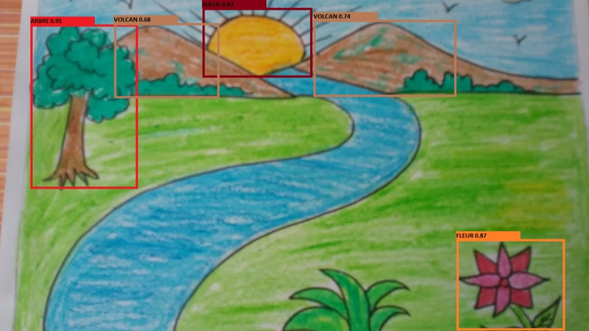
As we can see, some elements were not detected (the river, the grass in the foreground) and some were mislabeled (the two mountains perceived as volcanoes, probably due to the sunlight passing by). Our model can therefore be further improved, either by refining our database or by modifying the training parameters.

Optional: Split network training (when using the free version of Google Colab)

Although our use case remains simplistic, when using the free version of Google Colab, the training of our network can take several days before being completed. However, the restrictions of Google Colab (free version) prevent a program to run more than 12 hours. To keep the training, you just have to restart it after stopping a session with our last recorded weight as a parameter (weights):

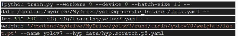
Here is an example launched with the 8th run (replace the folder "yolov78" by the last training done). You can find all your trainings in the associated folder in the Yolov7 tree.

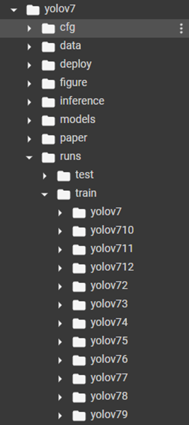
The training then resumes from the last epoch used, and allows you to progress without losing the time previously spent on your network.

References:

• Work, experiments and feedback from the R&D Lab.
• Contribution de WANG, Chien-Yao, BOCHKOVSKIY, Alexey, et LIAO, Hong-Yuan Mark. YOLOv7: Trainable bag-of-freebies sets new state-of-the-art for real-time object detectors. arXiv preprint arXiv:2207.02696, 2022. : https://arxiv.org/abs/2207.02696
• Official YOLOv7 code source : https://github.com/WongKinYiu/yolov7
• Microsoft COCO: Common Objects in Context : https://arxiv.org/pdf/1405.0312.pdf
• Create your model with YOLO https://datacorner.fr/yolo-custom-1/